A Follow-Up to Oil Prices and Inflation Expectations

Thinkstock/KCHL

This is a follow-up to “What Future Oil Price is Consistent with Current Inflation Expectations?” In the previous blog post, we concluded that, under several assumptions, “oil prices would need to fall to $0 per barrel by mid-2019 in order to validate current [breakeven] inflation expectations," as measured by the premium paid by standard Treasuries over inflation-protected Treasuries.

In this follow-up, we answer questions and requests contributed by several readers and market participants since February 23, when the post first appeared. First, we provide the oil price path that would validate current inflation expectations under the two alternative assumptions that the non-energy component of the consumer price index (CPI) grow at constant rates of either 2.18 or 1.99 percent. These are lower than our original assumption of 2.87 percent, which is the annualized growth rate of the all items less energy component between January 2014 and June 2014. We show that our conclusions are not dramatically affected under the alternative assumptions..

Second, we provide a formal description of our calculations. And, third, we provide a calculator in Excel (available here) that allows users to use their own assumptions and construct alternative scenarios.

Alternative Growth Rate for Nonenergy Components of CPI

The figures below provide two alternative assumptions for the growth of nonenergy CPI components, denoted g. The first figure displays results when g is 2.18 percent. This value corresponds to the annualized growth rate of the seasonally adjusted “all items less energy” component between December 2013 and June 2014. The second figure displays results when g is 1.99 percent. This value corresponds to the average annual growth rate of the unadjusted “all items less energy” component for the period 2005-15.

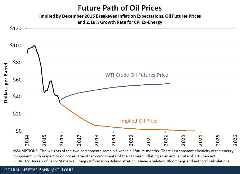
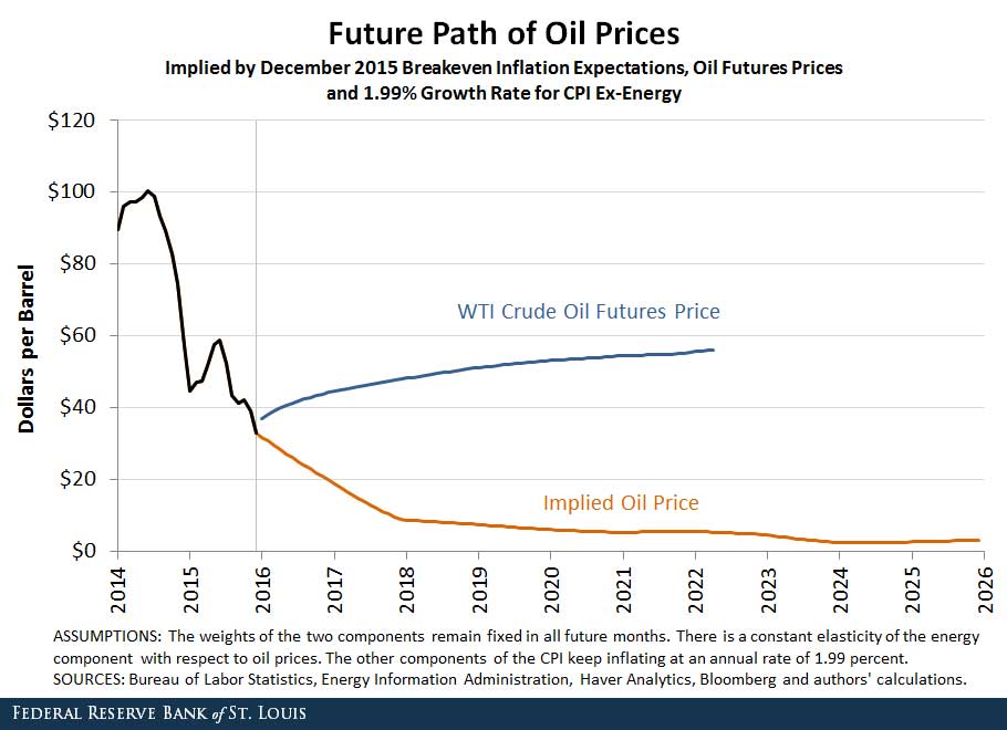
The figures show that the results do not vary dramatically with the assumption about the growth rate of CPI ex-energy. When this rate is 2.18 percent, the oil price series that would validate current breakeven inflation expectations reaches $0 by the end of 2024 instead of by mid-2019. When this growth rate is further reduced to 1.99 percent, oil prices do not need to be $0 to validate current breakeven inflation expectations, but they are required to fall to under $2.50 a barrel by 2024.

Additional Resources

• On the Economy: What Future Oil Price Is Consistent with Current Inflation Expectations?
• On the Economy: The Relationship between Wage Growth and Inflation
• On the Economy: Russia’s Economy Is Catching the U.S.’s, but It Has a Long Way to Go

Formal Description of Our Calculations

Consider inputs b_t+k, CPI_t, E_t and N_t, where b_t+k are breakeven rates for Treasuries maturing in k=1,2,…,10 years, CPI_t is the current value of the CPI, and E_t and N_t are the current values of the energy and nonenergy components of the CPI. We employ these inputs and the following four equations to construct a time series of future oil prices such that inflation expectations b_t+k are validated by the future path of oil prices:

(1)          CPI_t+k = αN_t+k + (1 – α)E_t+k,            k = 1, 2, …, 10

Equation (1) says that the CPI k years into the future is a weighted average of the nonenergy component N and the energy component E with fixed weight α. (The weight can be allowed to vary over time, which would require adding a fifth equation for the evolution of the weight.)

(2)          CPI_t+k = CPI_t(1 + b_t,k)^k,     k = 1, 2, …, 10

Equation (2) says that the CPI implied by the current breakeven rates, denoted CPI_t+k equals the current CPI, CPI_t, times the compound growth over k years implied by the breakeven inflation expectation b_t+k.

(3)          N_t+k = N_t(1 + g)^k,                k = 1, 2, …, 10

Equation (3) says that the nonenergy component, denoted N_t+k, grows at a constant rate g.

(4)          ln(E_t+k) = β₀ + β₁ln(P_t+k),                 k = 1, 2, …, 10

Equation (4) says that there is an elasticity β₁ of the energy component of the CPI, denoted E_t+k, and crude oil prices P_t+k for k=1, 2, …, 10.

The implied oil price is constructed as follows:

Use equation (2) to construct the future CPI series consistent with current breakeven rates. Construct the nonenergy component using equation (3). Exponentiate equation (4) to express the energy component as a function of oil prices.

(4’)         E_t+k = e^β0(P_t+k)^β1,                                k = 1, 2, …, 10

Plug the constructed CPI from equation (2), the nonenergy component from equation (3) and the energy component as a function of oil price from equation (4’) into equation (1), and call this equation (1’).

(1’)         CPI_t(1 + b_t,k)^k = αN_t(1 + g)^k + (1 – α)e^β0(P_t+k)^β1,     k = 1, 2, …, 10

Take equation (1’), and solve for oil prices. This gives the oil price that validates breakeven inflation expectations.

(1”)        P_t+k = ((CPI_t(1 + b_t,k)^k – αN_t(1 + g)^k) / (1 – α)e^β0)^1/β1,           k = 1, 2, …, 10

In our calculations we set the parameters of the model as follows:

• α = 0.92, the average relative importance of the all items less energy component from June 2015 to November 2015. (The December value was not yet available at the time of this analysis.)
• g = 1.99, 2.18 and 2.87 percent.
• β₁ =0.46, from estimating equation (4) using ordinary least squares from January 1995 to July 2015. See “predicting inflation.”
• β₀ = ln(E_t) – β₁ln(P_t), so that the relationship in equation (4) holds exactly in the last period with observable data