


Chained, Rested and Ready: The New and Improved GDP
Accurate estimates of U.S. gross domestic product (GDP) are a necessity. Why? Because the growth rate of GDP affects everything from presidential elections to a firm's sales forecast. If policymakers or business executives lack accurate estimates of economic growth, the decisions they reach will contain an element of error, which could then produce unintended consequences. To improve the measurement of real GDP—the broadest yardstick available for gauging the economy's performance—the U.S. Department of Commerce recently decided to compute GDP differently than the way it has in the past. Although the new measure of GDP, which took effect in January 1996, shows the economy to have grown more slowly over the past few years than originally thought, most economists have given it their stamp of approval.
Accounting for GDP
GDP is the capstone measure of the U.S. National Income and Product Accounts (NIPA). The NIPAs are an array of economic statistics designed to measure the production of goods and services and the income derived from the factors of production (land, labor and capital) that produce them. To calculate GDP, the Commerce Department collects millions of pieces of data from tax returns, census surveys and profit statements. These data, which are culled from households, businesses and government agencies, enable the department to construct a single measure of the dollar value of output produced in the United States every quarter. By definition, GDP counts only final goods and services—like the production of new cars, refrigerators and computers, or the services rendered by doctors, travel agents and hair dressers.1 Specifically, GDP is the sum of consumer spending on goods and services, investment expenditures by businesses (including any additions to inventory) and households, government purchases of goods and services, and the difference between exports and imports.
The problem with measuring the current dollar value of economic activity is that GDP will always rise as long as prices of goods and services rise. To properly analyze changes in economic activity, economists separate GDP into two parts: its price component and its quantity component. The price component of GDP refers to the prices of the millions of types of goods and services produced; the quantity component refers to the actual number of units produced. Thus, current dollar value of GDP—called nominal GDP—is simply price times quantity.
The quantity, or "real," measure of GDP is what most economists follow because it is an indication of the demand for goods and services produced. To construct real GDP, the current dollar value of its components are "deflated" by a series of price indexes and then "summed up."2 These price indexes are known as "fixed-weight" indexes because they measure changes in prices relative to a fixed base year, which Commerce would change about every five years.
Despite its familiarity, this measure of real GDP is flawed. Economists have known for quite a while that calculating real GDP using a fixed weighting scheme eventually produces substantial measurement error. There are two reasons for this. First, the structure of the economy—meaning the relative prices and types of goods and services produced—changes significantly over time.3 For example, think of the advent of the Internet and the products and services now offered online. Second, these relative price changes cause corresponding changes in the purchasing patterns of consumers. If, for instance, technological innovations lower the cost of producing a product, which should then lower its selling price, the quantity demanded of that product should increase and, accordingly, its importance in the calculation of GDP should increase.
Prior to the 1980s, the Commerce Department believed that these problems were not serious enough to warrant a change in the methodology used to calculate real GDP. The computer revolution, though, convinced them otherwise. In 1982, the production of information processing equipment (largely computers) as a share of GDP was 1.8 percent; by 1994, this share had more than doubled to 4.7 percent. At the same time, computer prices fell dramatically: Between 1982 and 1994, they dropped by roughly 13 percent a year. While a bonanza for consumers, these kinds of changes caused a significant problem for the number crunchers at Commerce.
The problem arises because the fixed-weighted system used to calculate GDP is not capable of fully accounting for these structural changes. As a result, the further the measure of GDP gets from the base year, the less accurate the calculation of real GDP becomes.
Under the old calculation method, the most recent base year was 1987. This meant that calculating real GDP in, say, 1994, was determined by: 1) how much the price of a particular good or service changed in relation to its price in 1987; and 2) how large a share it accounted for in relation to total GDP in 1987. To see how this works, let's use the example of the personal computer. According to the Commerce Department, today's Pentium personal computer would have cost about the same as what a new car cost in 1987—or, a little more than $13,700.4 In the fixed-weighted calculation of GDP, then, each new computer and new car produced added the same amount to GDP (about $13,700). By 1994, however, because of falling computer prices and rising new car prices, the average price of a new personal computer was around $2,500, while the price of a new car was almost $19,700. By calculating real GDP (in 1994) using fixed 1987 weights, however, each new computer was still being counted as if it were equal to one new car ($19,700) instead of its actual amount (about $2,500). This meant that fixed-weighted measures were overstating real growth in the output of computers and, thus, real GDP growth.
To counter this upward bias, the Commerce Department decided to estimate the quantity measure of GDP using a chain-weight system. Essentially, a chain-weight system differs from a fixed-weight system in that it measures output using current and previous year prices—something akin to a floating base year. For example, calculating chain-type GDP for 1994 is done using prices and quantities from 1993 and 1994.
Can the Chain-Weight Measure Up?
The primary advantage of the chain-weight measure is that it allows for substitution effects overtime—that is, it accounts for changes in consumption and production patterns that occur from relative price changes. Another important advantage is that chain-type measures value output of final goods and services for any period in terms of what the structure of the economy was at the time. Under the old method, Commerce would effectively rewrite economic history every time it reconfigured the GDP accounts to a different base year. Although the chain-weight measure of GDP depicts a more accurate portrayal of the business cycle, there are some drawbacks associated with using it. First, because of the way the chain-type measures are constructed, the components of GDP do not sum exactly to the total. In contrast, under the old method, GDP was the exact sum of its components. In percentage terms, however, this discrepancy is pretty small.
An ancillary problem that must be overcome concerns making economic forecasts with large-scale macroeconometric models. Under the old methodology, forecasters relied on the fact that GDP was the sum of its components. Because this is no longer strictly correct, forecasters will now be forced to restructure their models in away that introduces a greater potential for forecast error. While this hurdle may be eventually overcome through a process of learning-by-doing, it nevertheless introduces a further element of uncertainty that policymakers and others who closely monitor GDP forecasts must take into account.5 Despite these encumbrances, though, the new measure of GDP should more than measure up to its predecessor.
Difference In Real GDP Growth Using Fixed and Chain Weights
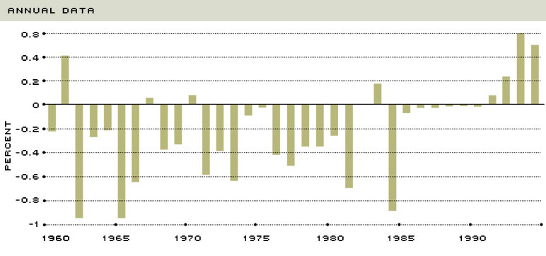
SOURCE: U.S. Department of Commerce
NOTE: The differences in real GDP growth rates over the 1960 to 1994 period using fixed weights and chain-type weights are illustrated in Figure 1. As expected, around 1987 the two rates were nearly identical because the fixed-weighted measures and the chain-type measures were using a similar base period. However, for the years before1987, the chain-weight measure shows real GDP to have increased more than the fixed weight measure—sometimes by nearly 1 percentage point per year. Conversely, since 1992 the fixed-weight measures of GDP have been increasing about 0.4 percentage points a year faster than the chain-weight measures. In the latter period, this was largely because the old method was improperly measuring computer output.
Endnotes
- To avoid double counting, real GDP is calculated using the value-added concept. This means, for example, that instead of adding up the total dollar value of all intermediate materials (like cotton) and labor used to produce a new shirt, their value is represented in the price of the shirt (the final good). [back to text]
- A price index, such as the consumer price index (CPI), attempts to aggregate into one number the prices of a large number of goods and services. For instance, in the NIPAs, a price index for personal consumption expenditures (PCE) is calculated, which attempts to measure the prices attached to everything from consumer spending on Big Macs to bib overalls. Similar price indexes are calculated for the other components of GDP. The real component of GDP is simply the current dollar value of each component of GDP divided by its respective price index. Real consumer spending, then, is the current value of spending divided by the PCE price index. [back to text]
- A relative price change occurs when the price of a good or service changes in relation to another. For example, if the price of hamburgers rises and the price of tacos stays the same, the relative price of hamburgers (to tacos) has risen. All other things equal, we should see people consume more tacos and fewer hamburgers. [back to text]
- See Ehrlich (1995). [back to text]
- See NABE News (1995). [back to text]
References
Ehrlich, Everett M. "The Statistics Corner: Notes on Chain-Weighted GDP," Business Economics (October 1995), pp. 61-62.
"Special Issue: Changes in the Reporting and Calculation of GDP," NABE News (September 1995).
Young, Allan H. "Alternative Measures of Change in Real Output and Prices," Survey of Current Business (April 1992), pp. 32-48.

Views expressed in Regional Economist are not necessarily those of the St. Louis Fed or Federal Reserve System.
For the latest insights from our economists and other St. Louis Fed experts, visit On the Economy and subscribe.
Email Us