Output Gaps, the Taylor Rule and the Stance of Monetary Policy

A 1993 study by John Taylor used a simple formula to describe the Federal Open Market Committee’s interest rate decision. In the formula, the gaps of inflation and real gross domestic product (GDP) relative to some reference levels determine what the Taylor rule considers to be the optimal federal funds rate.

Since the FOMC’s inflation target is 2% (an annual average over time), quantifying the gap concerning inflation is simple. When inflation is above 2%, the rule prescribes that the Fed increases the policy rate, and vice versa.

Calculating how the policy rate is affected by the output gap, however, is more complicated. Economists have suggested several ways of computing the real, or inflation-adjusted, gross domestic product’s deviation from its trend, also known as the “output gap.” This post discusses different output gap indicators and their implications for the stance of monetary policy under the Taylor rule.

Computing the Output Gap

There are different methods to compute the trend of GDP. Taylor’s original article used a trend that grew at 2.2% per year from 1984 to 1992. We employ a few adaptations of the technique proposed in a 1997 article by Robert Hodrick and Edward Prescott to characterize postwar U.S. business cycles.The simplicity of this method is ideal to facilitate the discussion here. However, it is known that the method has some undesirable properties, for example at the end points of the time series, as pointed out by James D. Hamilton’s 2018 article.

The Hodrick-Prescott (HP) filter selects the value of the trend at each period to minimize the sum of two terms. The first term equals the sum of the squared differences between the original series and the trend for every period. If only this term is considered, the resulting trend will be the same as the original series.

The second term is the sum of the squares of the differences in the trend component between periods t+1 and t for each period t. Thus, the higher the weight on this component (also known as a smoothing parameter), the closer the produced trend is to the least squares fit of a linear trend.

The period I examined begins in the first quarter of 1984, as John Taylor’s 1993 article did, and ends in the final quarter of 2023. The output gap is calculated by filtering the logarithm of real GDP per capita. I considered three different trends.

Linear Trend

The first trend is a linear trend. As previously stated, this case can be viewed as an HP filter with a very large smoothing parameter.

The Hodrick-Prescott Trend

The second trend is derived using the recommended smoothing parameter value of 1,600 for quarterly data, and it is referred to as the HP trend.

The Hodrick-Prescott Trend with Fitted Phillips Curve

This last trend includes a third term in the formula that is minimized to determine the trend values. This last term is the sum of the squared residuals from fitting a Phillips curve (PC) as shown in the 2017 article by Claudio Borio, Piti Disyatat, and Mikael Juselius.Equation 8 on page 673. When determining the trend, the intention is to consider the structural relationship between the output gap and inflation, which is often referred to as Phillips curve. This methodology would imply, for example, that given two periods with the same output level, the one with more inflation would be regarded as having a larger positive output gap (an economy with fewer idle resources). This trend is what I call the HP-PC trend.In this last case, since there is a new term, there is a weight associated with this term, which I set to 0.005. I also adjusted the weight in the second term such that the relative variance of the cycle is the same as with the HP trend.

The figure below shows the previously described three alternative series for output gaps. The blue line depicts the output gap calculated with a linear trend. The gap is wider in this case than in the other two since the trend’s growth rate remains constant. Surprisingly, the linear trend has been below zero (indicating that output is below its trend) practically every quarter since the global financial crisis (2007-9)— the lone exception is the final quarter of 2021.

The two gaps computed using the HP filter move together. During the recovery from the financial crisis, when inflation was low, the gray line—which represents the gap that adds a Phillips curve to the estimation—is lower than the orange line, which represents the gap from the HP filter alone. Keep in mind that from 2011 and 2019, the average annual inflation rate was 1.5%, as measured by the personal consumption expenditures price index. On the other hand, during the COVID-19 pandemic recovery, when inflation was more elevated, the gray line was higher. The average year-over-year inflation rate during 2021–2023 was 4.8%.

Alternative Estimates of the Output Gap

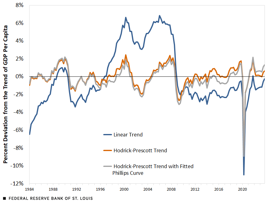
SOURCES: Bureau of Economic Analysis and author’s calculations.

How large are the differences in the three output gaps discussed above? Following John Taylor’s 1999 book, Monetary Policy Rules, I used his Rule IV with an output gap coefficient of 1.0 and an inflation gap coefficient of 1.5. In the Taylor formula, these coefficients mean that the prescribed policy rate—in the case of the U.S., the federal funds rate targeted by the FOMC to conduct monetary policy—should react one-to-one to deviations in output gap and by 50% more to deviation in inflation from its target.For example, a coefficient of 1.0 means that if the output gap increases by 1 percentage point (e.g., the deviation from the trend rises from 2% to 3%), the optimal policy rate should increase by 1 percentage point. I considered the full year 2023 to avoid placing too much emphasis on the last observed quarter.

The difference among the averages of the output gaps for 2023 is 1 percentage point, which, due to our assumption on the coefficient of the Taylor rule, imply a 1 percentage point difference among the prescribed interest rates. Moreover, adding the assumption of a 2% “equilibrium” real rate as in Taylor’s 1993 article, these gaps imply average interest rates for 2023 of 4.2%, 4.8%, and 5.2% for the gaps computed using the linear, HP and HP-PC trends, respectively.

Overall, these estimates reveal that the indicators of output gaps suggest different prescribed interest rates for 2023. This uncertainty is in line with the challenges in using the output gap to gauge the stance of monetary policy, as outlined in Thomas A. Lubik and Stephen Slivinski’s 2010 essay. Although calculating these rates remains mostly a theoretical exercise, note that the average of the three prescribed rates for 2023 is slightly lower but still close to the effective fed funds rate, which was approximately 5% on average in 2023.

Notes

1. The simplicity of this method is ideal to facilitate the discussion here. However, it is known that the method has some undesirable properties, for example at the end points of the time series, as pointed out by James D. Hamilton’s 2018 article.
2. Equation 8 on page 673.
3. In this last case, since there is a new term, there is a weight associated with this term, which I set to 0.005. I also adjusted the weight in the second term such that the relative variance of the cycle is the same as with the HP trend.
4. For example, a coefficient of 1.0 means that if the output gap increases by 1 percentage point (e.g., the deviation from the trend rises from 2% to 3%), the optimal policy rate should increase by 1 percentage point.