How Much Are We “Taxed” by Surprise Inflation?

In an economy, borrowing and lending are typically conducted in nominal terms: A lender provides a loan for a certain sum of money and a borrower repays that exact sum plus interest. This means that, whenever the price level of goods and services is different from what people expected—an “inflation shock”—each transaction has a “winner” and a “loser” in terms of the real value delivered (in comparison to what was agreed upon).

In particular, when inflation turns out to be higher than expected (a positive inflation shock), then what the borrower needs to repay will be much less valuable than what was expected when the agreement was made, that is, a positive inflation shock benefits nominal borrowers at the expense of lenders.

The U.S. government is one of the largest of these nominal borrowers in the world. Over the past 40 years, the nominal U.S. government outstanding debt averaged around 57% of U.S. gross domestic product (GDP). In this article, we used inflation expectation data from the Cleveland Fed to calculate inflation surprises over the past four decades, and together with data on U.S. Treasury debt from the Center for Research in Security Prices, we provide a back-of-the-envelope calculation of how much the U.S. government gains and loses from inflation shocks.

With total U.S. government debt increasing to more than 100% of U.S. GDP last year and with the large surprise increase in inflation in 2021, the U.S. government is a big winner. The decrease in the real value of debt amounts to 3.3% of U.S. GDP—at the expense of the debtholders, who were effectively hit by a 6.5% tax on the wealth held in nominal Treasury.

Inflation Shocks: From 1984 to 2021

The Cleveland Fed provides estimates of inflation expectations each month over different horizons.These values are computed by a model based on Treasury yields, inflation data, inflation swaps, and survey-based measures of inflation expectations. For each year, we calculate how much the initial expectation has changed over the course of one year because of new information about the economy. For example, if last year you expected inflation to be 2%, but actual inflation over the year turns out to be 4%, then that is an inflation shock of 2 percentage points.

Similar logic can be applied to longer horizons as well. For example, if last year (say, January 2021) you expected inflation to be 2% per year on average for the next five years (the period January 2021 to January 2026), but with new information that arrived over the previous year, now today, in January 2022, you update your inflation expectations for the same period (January 2021 to January 2026) to average 4% instead. That represents an inflation shock of 2 percentage points annually for the five-year horizon.

In the next figure, we plotted the annualized inflation shocks in the United States over five different horizons.

Annualized U.S. Inflation Shocks for Various Time Horizons

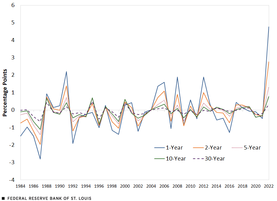
SOURCES: Federal Reserve Bank of Cleveland and authors’ calculations.

NOTES: The data represent the percentage point change in expected inflation over the course of a year for different horizons. Expectations are set on Jan. 1 of each year.

The inflation shock people experienced in 2021 was the largest over the last four decades in terms of one-year, two-year, five-year and 10-year horizons, while the shock to 30-year horizons is the largest since 2000.

To illustrate how inflation shocks redistribute between borrowers and lenders of nominal contracts, consider the following example: Suppose you are wanting to buy a car that costs $10,000 today. You agree to borrow the $10,000 from your bank today and pay it back, with 5% interest—for a total of $10,500—one year from today. Suppose the bank and you both expect inflation to be zero percent. However, if after a year, realized inflation turns out to be 10%, then the $10,500 you promised to pay is worth only $9,450 in today’s dollars [$10,500 – ($10,500 × 0.1)], and you are actually paying back less than the principle you borrowed.

This example illustrates the redistributive effect of surprises in inflation. This phenomenon also holds for longer horizon shocks—the original value of contracts changes when agreements are made based on the expected cumulative inflation rate over the agreed horizon, and the market updates its expectation over time with the arrival of new information.

U.S. Treasury Debt

The U.S. government is one of the largest nominal borrowers in the world. This means the same redistribution happens between the U.S. government and its debtholders when the U.S. government borrows money in nominal terms today and pays it back at agreed-upon dates in the future.

Rather than a single lump-sum payment, as in the earlier example, Treasury securities mature in a wide range of horizons. To understand how Treasury debts of different maturities are exposed to inflation shocks, we calculate, for each year, the year-end nominal value of Treasury debt that is outstanding and priced at the beginning of each year.We exclude debt held by the Federal Reserve.

Consider an example: If in January 2021, the U.S. government needs to make a payment of $10,500 in one year, in January 2022, and $10,500 in two years, in January 2023, and the market nominal interest rate (the forward rate) is expected to be 5% between January 2022 and January 2023; then in January 2021, the year-end value for the one-year horizon is $10,500, and the year-end value for the two-year horizon is $10,000 ($10,500/1.05).

These values represent the year-end amounts the U.S. government agrees to pay in January 2021 that are exposed to inflation shocks, and they allow us to understand how changes in the real value of nominal amounts from over the year affect the real value of outstanding debt of different horizons that the U.S. government had promised to pay—that is, how inflation shocks of different horizons affect the total real value of the U.S. government debt.

In the next figure, we plotted the year-end nominal value of Treasury debt as a percentage of nominal GDP by payment horizons, for all Treasury debt due in one year or further. As shown in the figure, the largest share of current outstanding Treasury debt is debt maturing in three to five years, followed closely by two-year maturities. This means that the two-year and five-year inflation expectation shocks will have the largest redistributive impact on the government budget.

Breakdown in the Nominal Value of U.S. Treasury Debt at Year-End

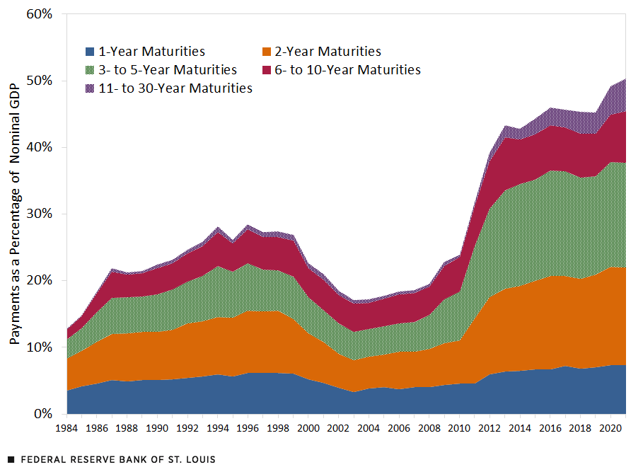
SOURCES: Center for Research in Security Prices and authors’ calculations.

NOTE: The stacked areas represent the composition of payments of different maturities.

The Implied “Inflation Tax”

How do inflation surprises affect the real value of Treasury debt? Suppose that in January 2021, when people agreed to lend money to the government, inflation was expected to be zero percent for the next two years; to keep this example simple, we also assume a forward rate of zero. However, over the first year, inflation was actually 5%, and people now expect inflation to average 3% in the two-year horizon: an inflation shock of 5% for the one-year horizon and 1% for the second year. As a result, payment of $1 at the end of the first year loses around 4.76% of its originally expected value (-4.76% ≈ 1/1.05 − 1), and a payment at the end of the second year with value of $1 loses around 5.7% of its originally expected value (-5.7% ≈ 1/1.03² − 1).

If we apply the logic from the previous example to a larger scale, in January 2021, the government promised two payments with one- and two-year maturities to bond holders that have nominal value equivalent to $1.6 trillion and $3.15 trillion respectively in January 2022. With these amounts, the inflation shocks considered above for the one- and two-year horizons will lead to a 4.76% decrease in real value for the first payment—a loss of $76.2 billion ($1.6 trillion ×4.76%)—and a decrease of 5.7% for the second payment—for a loss of $179.55 billion ($3.15 trillion ×5.7%)—relative to their original values. Following this logic, we calculate how inflation shocks redistribute between the U.S. Treasury and its debtholders each year.

In the next figure, we plotted how much inflation surprises have decreased the real value of U.S. government debt as a percentage of U.S. GDP each year over the previous four decades. A positive number means a redistribution from debtholders to the U.S. government, an inflation tax on the debt holders.

Size of the Annual Inflation Tax on U.S. Treasury Debtholders

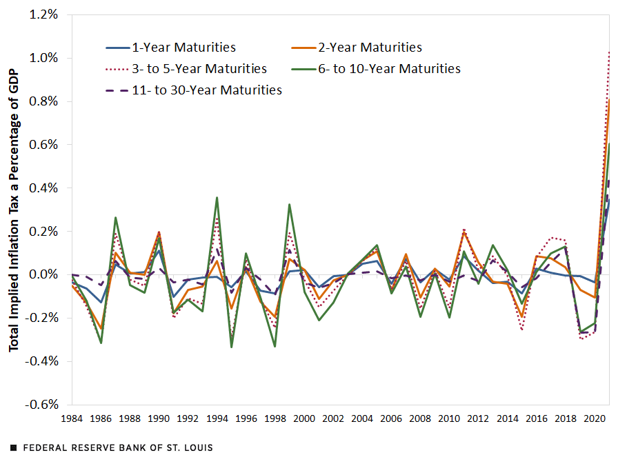
SOURCES: Center for Research in Security Prices, Federal Reserve Bank of Cleveland and authors’ calculations.

Historically, the effects of inflation shocks, both positive and negative, have been small—barely exceeding 1% of U.S. GDP in the most extreme cases. However, the large inflation surprises we experienced last year, together with the ever-increasing Treasury debt in recent years, has led to an unprecedented, large-scale redistribution. This has resulted in an inflation tax that amounts to 3.3% of U.S. GDP imposed on Treasury debtholders—that is, a tax rate of 6.5% on wealth invested in Treasury securities due in one year or further. While 38% of the Treasury debt, not counting that which is held by the Federal Reserve, is owned by foreigners, nearly 62% of this debt is held by U.S. households, either directly or indirectly, according to the most recent release of the Financial Accounts of the United States.

Conclusion

The federal government is the largest nominal debtor in the economy. This means it is either the biggest winner or loser from every inflation shock. With the unprecedented positive inflation shock we have experienced over the last year, the federal government has come out as a big winner, with an inflation tax that amounts to around 3.3% of GDP, equivalent to a 6.5% tax on wealth held in Treasury securities. These numbers can be expected to change if there are more surprises in inflation.

Notes and References

1. These values are computed by a model based on Treasury yields, inflation data, inflation swaps, and survey-based measures of inflation expectations.
2. We exclude debt held by the Federal Reserve.