Quantitative Easing: How Well Does This Tool Work?

Quantitative easing (QE)—large-scale purchases of assets by central banks—led to a large increase in the Federal Reserve’s balance sheet during the global financial crisis (2007-2008) and in the long recovery from the 2008-2009 recession. Over the same period, QE played a very important role at other central banks in the world. Indeed, in some of those countries, particularly Japan, QE remains a key instrument of monetary policy—an unconventional policy tool that central bankers can potentially use when all else fails. Public policy discussion suggests that QE is likely to be used again, by the Fed and other central banks, in a future recession or financial crisis. Thus, at this juncture it is useful to evaluate what we know about QE. How is it supposed to work, and does it work as advertised?

QE consists of large-scale asset purchases by central banks, usually of long-maturity government debt but also of private assets, such as corporate debt or asset-backed securities. Typically, QE occurs in unconventional circumstances, when short-term nominal interest rates are very low, zero or even negative.

The first high-profile use of QE seems to have been the Bank of Japan program that began in 2001. Then, during and after the international financial crisis, the use of QE became much more widespread, used by central banks in the U.S., the U.K., the euro area, Switzerland and Sweden, for example.

QE is controversial, the theory is muddy and the empirical evidence is open to interpretation, in part because there is little data to work with. The purpose of this article is to review the key features of QE and how it has been used, to explain and evaluate the available theory of QE, and to provide a critical review of the empirical work. Also discussed are two natural experiments that shed light on how QE works (or does not work).

What Is Quantitative Easing?

QE is an unconventional monetary policy action, in a class with forward guidance and negative nominal interest rates. To understand QE, we first need to review how conventional monetary policy works.

Conventional monetary policy is about the choice of the target for the short-term nominal interest rate and how that interest rate target should depend on observations concerning aggregate economic performance. Formally, some macroeconomists characterize central banks as adhering to a Taylor rule,¹ which specifies that the central bank’s nominal interest rate target should go up if inflation exceeds the central bank’s inflation target (2 percent for the Fed) and that the nominal interest rate target should go down if aggregate output (measured, say, by real gross domestic product [GDP]) falls below what is deemed to be the economy’s potential.

But there is a limit to how low the short-term nominal interest rate can go—the so-called effective lower bound. In the U.S., this effective lower bound may be essentially zero, but in some other countries the effective lower bound is negative. For example, the central banks in Sweden, Denmark, Switzerland and the euro area have implemented negative short-term interest rates.

Traditionally, the interest rate that the Fed targets is the federal funds (fed funds) rate. Suppose, though, that the fed funds rate target is zero, but inflation is below the Fed’s 2 percent target and aggregate output is lower than potential. If the effective lower bound were not a binding constraint, the Fed would choose to lower the fed funds rate target, but it cannot. What then? The Fed faced such a situation at the end of 2008, during the financial crisis, and resorted to unconventional monetary policy, including a series of QE experiments that continued into late 2014.

In essentially all of the QE programs conducted in the world during and after the financial crisis, central banks seemed primarily interested in how the type and quantity of asset purchases would affect financial market conditions and, ultimately, inflation and aggregate economic activity. For example, on Nov. 25, 2008, the Fed announced its first QE program, sometimes called QE1. The press release concerning the program provided detail on the types of assets that the Fed would purchase—agency debt and mortgage-backed securities issued by government-sponsored enterprises (GSEs)—along with the dollar amounts that would be purchased.² As well, the announcement made clear that the intent of the program was to affect general financial conditions and, more specifically, the housing and mortgage markets.

Further QE programs implemented by the Fed were, if anything, more specific about the nature of the purchases:

1. QE1, December 2008 to March 2010: Purchases of $175 billion in agency securities and $1.25 trillion in mortgage-backed securities.
2. Reinvestment Policy, August 2010 to present: Replacement of maturing securities to maintain the balance sheet at a constant nominal size if there is no QE program underway.
3. QE2, November 2010 to June 2011: Purchases of $600 billion in long-maturity Treasury securities.
4. Operation Twist, September 2011 to December 2012: Swap of more than $600 billion involving purchases of Treasury securities with maturities of six to 30 years and sales of Treasury securities with maturities of three years or less.
5. QE3, September 2012 to October 2014: Purchases of mortgage-backed securities and long-maturity Treasury securities, initially set at $40 billion per month for mortgage-backed securities and $45 billion per month for long-maturity Treasury securities.

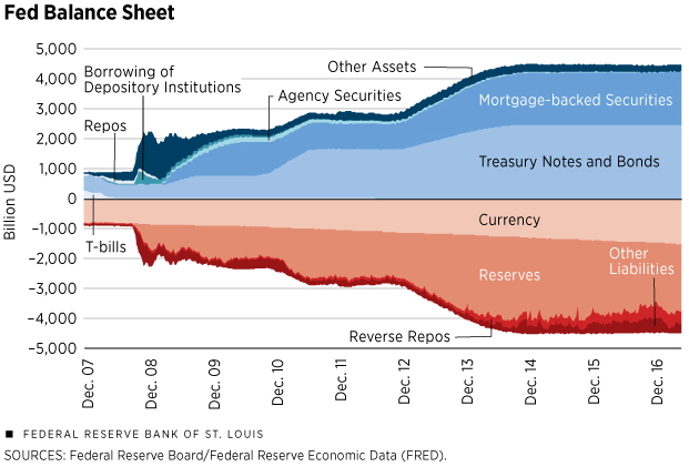
The implications of all of these programs for the Fed’s balance sheet can be observed in Figure 1. From December 2007 to May 2017, the Fed’s total assets increased from $882 billion to $4.473 trillion—a fivefold increase. To give a measure of the magnitude of the program, total Fed assets increased from 6.0 percent of U.S. GDP in the fourth quarter of 2007 to 23.5 percent of GDP in the first quarter of 2017. Further, the average maturity of the assets in the Fed’s portfolio in early 2017 was much higher than before the financial crisis. As of May 2017, the Fed held no Treasury bills, which mature in a year or less; the Fed’s security holdings consisted almost entirely of long-maturity Treasury securities and mortgage-backed securities.

Other central banks have been actively engaged in QE since the financial crisis—some in a bigger way than the Fed. For example, in December 2016 the Bank of Japan had a balance sheet that was 88 percent of GDP, Switzerland’s was 115 percent of GDP, the Swedish Riksbank’s was 19 percent of GDP, the Bank of England’s was 24 percent of GDP and the European Central Bank’s was 34 percent of GDP.³

What is a typical central bank justification for QE? How do central bankers think these policies work? At the 2010 Jackson Hole conference, then-Fed Chairman Ben Bernanke attempted to articulate the Fed’s rationale for QE.⁴ Bernanke’s view was that, with short-term nominal interest rates at zero, purchases by the central bank of long-maturity assets would act to push up the prices of those securities because the Fed was reducing their net supply. Thus, long-maturity bond yields should go down, for example, if the Fed purchases long-maturity Treasury securities. Bernanke then argued that this was “accommodation,” in the same sense as a reduction in the fed funds rate target is accommodation. Thus, QE should be expected to increase inflation and aggregate real economic activity.

Conventional Theory of QE

What macroeconomic theory has been brought to bear in evaluating the efficacy of QE? In conventional policy discourse, there are three basic theories: portfolio balance or segmented markets theory, preferred habitat theory, and signaling.

First, with respect to portfolio balance theory, when central bankers use QE, they appear to believe that purchases of long-maturity assets will make the yield curve flatter.⁵ That is, with short-term interest rates at zero, or close to it, declines in long-term interest rates will narrow the margin between long-term and short-term rates. According to portfolio balance theory, assets of different maturities are imperfect substitutes because of frictions that inhibit arbitrage across maturities—assets are costly to buy and sell, for example. This, then, implies that the relative supplies of assets matter—a lower supply of long-term assets and a higher supply of short-term assets imply that long-term interest rates fall and short-term interest rates rise.

Second, preferred habitat theory posits that financial market participants have preferences over maturities of assets.⁶ For example, life insurance companies have long-maturity liabilities; to hedge risk, these financial intermediaries have a preference for long-maturity assets. This implies a type of asset market segmentation, making the mechanism by which QE might work similar to portfolio balance theory.

Third, in signaling theory, even if there are no direct effects of quantitative easing, commitment to future monetary policy can matter for economic outcomes in the present, and quantitative easing may be a means for the central bank to commit. That is, the structure of the central bank’s current asset portfolio may bind future monetary policymakers to particular actions.⁷

An Alternative Approach to QE Theory

A central bank is a financial intermediary. It borrows from a large set of people—those who hold the central bank’s primary liabilities, i.e., currency and reserves. And the central bank lends to the government, private financial institutions and sometimes to private consumers. (For example, the Fed indirectly holds private mortgages, which back the mortgage-backed securities in its portfolio.)

Like private financial intermediaries, central banks transform assets in terms of maturity, liquidity, risk and rate of return. Therefore, the ability of a central bank to affect economic outcomes in a good way depends on its having an advantage relative to the private sector in intermediating assets. Perhaps surprisingly, none of the theories typically used by central bankers to justify QE—portfolio balance (segmented markets), preferred habitat, signaling—integrates financial intermediation into the analysis in a serious way.

To see how financial intermediation theory is important for understanding monetary policy, consider how conventional monetary policy works. The primary liabilities of a central bank are currency and reserves, which play important medium-of-exchange roles in retail transactions and in transactions among financial institutions. But we could imagine monetary systems in which the media of exchange used in transactions are the liabilities of private financial institutions, and those financial institutions create their own cooperative arrangements for executing transactions among themselves. Indeed, before the Fed opened its doors in 1914, much of the currency issued in the U.S. consisted of private bank notes.

Those notes were issued by state-chartered banks during the free banking era (1837-1863) and by nationally chartered banks during the national banking era (1863-1913). From 1824 to 1858, one arrangement for interbank transactions was the Suffolk banking system, which operated in New England. Another example of a private monetary system was the pre-1935 note-issue system in Canada, under which chartered banks issued circulating notes and the Bank of Montreal (a private bank) acted as a quasi-central bank.

So, given historical precedent, the current functions of central banks could, in principle, be carried out by the private financial system. But there is a presumption that such an arrangement would be less efficient than having a central bank.

Indeed, in the U.S., it was decided in the early 20th century that relying on private monetary arrangements is a bad idea. The argument, enshrined in the Federal Reserve Act of 1913, is that, in the absence of a central bank, the financial sector would be unstable and would be insufficiently responsive to fluctuations in the need for financial intermediation. The Fed was designed to stabilize the financial sector through discount-window lending in crises and to accommodate fluctuating needs for currency.

The foundation for monetary policy rests on the central bank’s uniqueness as a financial intermediary. In the case of the U.S., in pre-financial crisis times, the Fed’s liabilities consisted mainly of currency and a relatively small quantity of reserves, and its assets were mainly Treasury securities. Thus, the Fed was primarily transforming the debt of the U.S. Treasury into currency. Given the Fed’s monopoly on the supply of currency, and since private-sector bank deposits are imperfect substitutes for currency, if the Fed conducted an open market operation—say a swap of reserves for Treasury bills—then this would matter. That is, through movements in market interest rates and portfolio adjustments by financial institutions and consumers, the new reserves created by the open market purchase would end up as currency. Thus, the Fed would have increased the quantity of intermediation it was doing, in nominal terms. Because this central bank financial intermediation was not offset by less private-sector financial intermediation of the same type, there would be effects on asset prices, inflation and aggregate economic activity.

But QE is fundamentally different from conventional open market operations. QE is conducted in a financial environment in which there are excess reserves outstanding in the financial system. Given the interest rate on excess reserves (IOER), other interest rates and quantities adjust so that banks are willing to hold the reserves supplied by the central bank. It is generally recognized that a financial system flush with reserves, as has been the case in the U.S. since late 2008, is subject to a liquidity trap. That is, given IOER, which is set administratively, if the Fed simply swaps reserves for Treasury bills, then this may have no effect because reserves and Treasury bills might be viewed as roughly identical short-term assets.

Indeed, such a swap may even have negative effects, as reserves may be inferior assets to Treasury bills.⁸ For example, on May 19, 2017, the one-month Treasury bill rate was 0.71 percent while IOER was 1.00 percent, so banks required a premium of 29 basis points to induce them to hold reserves rather than one-month T-bills. For what reasons are reserves inferior to T-bills? Basically, reserves can be held only by a restricted set of financial institutions, while T-bills are more widely held and are useful as collateral in financial transactions (e.g., repurchase agreements) in ways that reserves are not.

When QE is conducted in a system flush with reserves, the central bank is typically transforming long-maturity assets into short-maturity reserves. The key question, if we compare this to how conventional monetary policy works, is what advantage the central bank might be exploiting in conducting such a transformation. That is not clear. Consider, for example, a shadow bank (an unregulated financial institution that conducts bank-like activities) that holds long-maturity assets—Treasury bonds, for example—and finances its portfolio by rolling over overnight repurchase agreements (repos), with the Treasury bonds serving as collateral. This looks much like the asset transformation in QE, except it might actually be more efficient because overnight repos may be superior assets to reserves for the same reason that T-bills may be superior to reserves.

Therefore, from financial intermediation theory, it is not clear that QE should have any effect and it might actually be detrimental to the efficiency of the financial system. Some economists have made the case that QE has negative effects, due to the fact that it withdraws safe collateral from financial markets, thus clogging up the “financial plumbing.” ⁹ On the theoretical side, it has been shown that QE can have beneficial effects, provided that reserves and short-term government debt are identical, and long-maturity government debt is better collateral than short-term government debt.¹⁰ However, it has also been shown that balance-sheet expansion by the central bank can be detrimental if reserves are inferior to short-term government debt.¹¹

Empirical Evidence on QE

The empirical work evaluating the effects of QE was summarized nicely by two other economists last year.¹² For the most part, QE empirical studies fall into one of three categories: (1) event studies, (2) regression and VAR (vector autoregression) evidence, and (3) calibrated model simulations. The weight of the results was interpreted by those economists as favoring the standard central banking narrative concerning QE. That is, according to the narrative, QE works much as conventional accommodative policy does—it lowers bond yields and increases spending, inflation and aggregate output.

But we should be skeptical of this interpretation. First, event studies look at the reaction of asset prices in a short window around a policy announcement. But the fact that asset-market participants respond in the way that policymakers hope they respond to a policy announcement with little historical precedent may say very little. Second, the two economists of this study pointed out plenty of econometric problems in the studies they surveyed. Third, none of this empirical work actually measured the advantage that central banks might have in transforming assets when they conducted QE.

Natural Experiments

Primarily, we are interested in how QE matters for the ultimate goals of central banks—generally pertaining to inflation and real economic activity. One type of empirical evidence to which we can appeal is so-called natural experiments—instances in which the policy was tried and the effects are more-or-less obvious. We will look at two cases: (1) QE in Japan post-2013, and (2) Canada and the United States after the financial crisis.

In January 2013, the Bank of Japan (BOJ) announced that it would pursue a 2 percent inflation target, and in April 2013 it announced the Quantitative and Qualitative Monetary Easing Program, intended to achieve the 2 percent target within two years. From 2013 to early 2016, the overnight nominal interest rate was close to zero, and it has been negative since early 2016. In Figure 2, note that the monetary base in Japan (a measure of total liabilities of the Bank of Japan) increased by about threefold from the beginning of 2013 to May 2017.

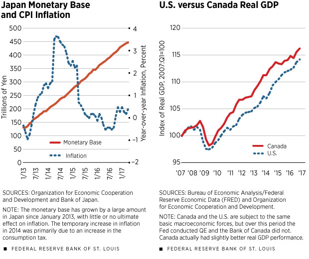
If QE is indeed effective in increasing inflation—the BOJ’s ultimate goal—then surely inflation should have increased in response to this massive QE program. But Figure 2 shows that this was not the case, if we look at the consumer price index (CPI) for Japan. CPI indeed increased in 2014, but largely due to an increase of three percentage points in Japan’s consumption tax in April 2014, which fed directly into the CPI measure. But, from mid-2015 to March 2017, average inflation in Japan was roughly zero, obviously far short of the 2 percent target.

Since the financial crisis, central bank interest rate policy has been little different in Canada and the U.S. But, the Bank of Canada did not engage in QE over this period, while the Fed did. As of December 2016, the Bank of Canada’s balance sheet stood at 5.1 percent of GDP, as compared to 23.6 percent of GDP for the Fed. Canada and the United States are typically subject to similar economic shocks, given their close proximity and similar level of economic development; so, if QE were effective in stimulating aggregate economic activity, we should see a positive difference in economic performance in the U.S. relative to Canada since the financial crisis. In Figure 3, we show real GDP in Canada and the United States, scaled to 100 for each country in the first quarter of 2007. The figure shows that there is little difference from 2007 to the fourth quarter of 2016 in real GDP performance in the two countries. Indeed, relative to the first quarter of 2007, real GDP in Canada in the fourth quarter of 2016 was 2 percent higher than real GDP in the U.S., reflecting higher cumulative growth, in spite of supposedly less accommodative monetary policy.

Thus, in these two natural experiments, there appears to be no evidence that QE works either to increase inflation, if we look at the Japanese case, or to increase real GDP, if we compare Canada with the U.S.

Conclusion

Evaluating the effects of monetary policy is difficult, even in the case of conventional interest rate policy. With unconventional monetary policy, the difficulty is magnified, as the economic theory can be lacking, and there is a small amount of data available for empirical evaluation. With respect to QE, there are good reasons to be skeptical that it works as advertised, and some economists have made a good case that QE is actually detrimental.

One way of viewing QE is that it represents an asset transformation by the central bank; for example, the central bank turns long maturity government debt into short maturity reserves. Two questions then arise.

First, the fiscal authority could have done the same thing by issuing less long-maturity debt and more short-maturity government debt. So, is the case for QE that the central bank is somehow better at debt management than the fiscal authority? If so, there should be an explicit agreement between the government and the central bank concerning who possesses the power to manage the maturity structure of outstanding debt.

Second, perhaps the private sector can do a better job than the central bank in turning long-maturity debt into short-maturity debt. If that is the case, then perhaps the central bank should be permitted to issue a richer set of liabilities—circulating debt similar to Treasury bills for example, which would be superior as an asset to bank reserves. Indeed, the central banks in Switzerland and China already have the power to issue such central bank bills.

Stephen Williamson is an economist at the Federal Reserve Bank of St. Louis. For more of his work, see https://research.stlouisfed.org/econ/williamson. Research assistance for this article was provided by Jonas Crews, a senior research associate at the Bank.

Endnotes

1. See Taylor. [back to text]
2. See Board of Governors. [back to text]
3. For the euro area, we counted GDP as a measure of total GDP for the countries that are members of Europe’s Economic and Monetary Union. [back to text]
4. See Bernanke. [back to text]
5. For examples of this theory, see Tobin, as well as Vayanos and Vila. [back to text]
6. For examples, see Modigliani and Sutch. [back to text]
7. Such arguments have been made by Woodford and by Bhattarai et al. (2015). [back to text]
8. See Williamson (2017). [back to text]
9. See Singh and Stella. [back to text]
10. See Williamson (2016). [back to text]
11. See Williamson (2017). [back to text]
12. See Bhattarai and Neely (2016). [back to text]

References

Bernanke, Ben. The Economic Outlook and Monetary Policy. Speech at the Federal Reserve Bank of Kansas City Economic Symposium, Jackson Hole, Wyo., Aug. 27, 2010.

Bhattarai, Saroj; and Neely, Christopher. A Survey of the Empirical Literature on U.S. Unconventional Monetary Policy. Federal Reserve Bank of St. Louis working paper 2016-021A, October 2016.

Bhattarai, Saroj; Eggertsson, Gauti; and Gafarov, Bulat. Time Consistency and the Duration of Government Debt: A Signalling Theory of Quantitative Easing. National Bureau of Economic Research (NBER) working paper 21336, July 2015.

Board of Governors of the Federal Reserve System. Press release, Nov. 25, 2008. See www.federalreserve.gov/newsevents/press/monetary/20081125b.htm.

Modigliani, Franco; and Sutch, Richard. Innovations in Interest Rate Policy. American Economic Review, March 1966, Vol. 56, pp. 178-97.

Singh, Manmohan. Collateral and Financial Plumbing, Second Impression. Risk Books, 2016.

Stella, Peter. Condensing the Fed’s Balance Sheet is as Simple as This. Stellar Consulting: A Research Blog, February 2017. See stellarconsultllc.com/blog/wp-content/uploads/2017/02/Condensing-the-Fed-Balance-Sheet-is-as-Simple-as-This-1.pdf.

Taylor, John. Discretion versus Policy Rules in Practice. Carnegie-Rochester Conference Series on Public Policy, 1993, Vol. 39, pp. 195-214.

Tobin, James. A General Equilibrium Approach to Monetary Theory. Journal of Money, Credit, and Banking, Vol. 1, 1969, pp. 15-29.

Vayanos, Dimitri; and Vila, Jean-Luc. A Preferred-Habitat Model of the Term Structure of Interest Rates. NBER working paper 15487, November 2009.

Williamson, Stephen. 2016. Scarce Collateral, the Term Premium, and Quantitative Easing, Journal of Economic Theory, 2016, Vol. 164, pp. 136-65.

Williamson, Stephen. 2017. Interest on Reserves, Interbank Lending, and Monetary Policy, Federal Reserve Bank of St. Louis working paper.

Woodford, Michael. Methods of Policy Accommodation at the Interest Rate Lower Bound. The Changing Policy Landscape: 2012 Jackson Hole Symposium, Federal Reserve Bank of Kansas City, 2012, pp. 185-288.