

Tightening Monetary Policy and Patterns of Consumption
KEY TAKEAWAYS
- In theory, tightening monetary policy makes credit more expensive, which reduces consumption and investment and—in turn—works to lower inflation as firms adjust prices.
- An analysis covering five episodes of monetary policy tightening since 1990 shows there is some evidence, albeit weak, that personal consumption declines in such periods.
- Consumption was consistently about 2% above trend in 2022 despite tightening monetary policy. More recently, this could be a consequence of an improvement in financial conditions.
Throughout business cycles—periods of recession and expansion—the Federal Reserve raises and lowers interest rates to achieve its mandate of stable prices and maximum sustainable employment. When the Fed increases interest rates, it is said to be “tightening” monetary policy. A higher interest rate may help control high inflation because, the theory suggests, access to credit becomes more expensive (i.e., financial conditions tighten), which reduces consumption and investment. In turn, firms adjust prices and inflation falls.This logic is close to the description of the Phillips curve in this May 2020 working paper from the European Central Bank (PDF).
In this article, we analyze the connection between the effective monetary policy rate and the consumption of goods and services during the last five episodes of monetary policy tightening, emphasizing the most recent experience.
Measuring the Monetary Policy Rate at the Zero Lower Bound
The federal funds rate is the target interest rate set by the Federal Open Market Committee for overnight loans between banks. Although the Fed conducts monetary policy primarily through the federal funds rate, it must use other tools if it wants additional stimulus when the federal funds rate nears zero. This is because central banks find it difficult to push short-term interest ratesShort-term rates are those with maturity less than one year. The federal funds rate is a short-term rate. below zero, as people can decide to hold cash rather than to lend money at negative interest rates. Therefore, when short-term rates hit zero, the Fed employs other tools, such as bond purchases, that push down medium- and long-term rates to stimulate economic activity, a method known as quantitative easing.
Comparing monetary stimulus from policies like quantitative easing to that from ordinary short-term interest rate levels is difficult because short-term rates don’t reflect the stimulus from quantitative easing. To make such a comparison easier, economists Jing Cynthia Wu and Fan Dora Xia estimated a “shadow rate” that describes the hypothetical short-term rate which would provide the same stimulus as the quantitative easing being applied.See their paper, “Measuring the Macroeconomic Impact of Monetary Policy at the Zero Lower Bound,” published in the March 2016 issue of the Journal of Money, Credit and Banking.
We define the effective monetary policy rate (the dotted black line in the figure below) as the effective federal funds rate (the blue line) above the zero lower bound. The effective monetary policy rate is defined as the shadow rate (the yellow line) when the effective federal funds rate is at the zero lower bound. The gray bars indicate episodes of monetary policy tightening.We focus on five tightening episodes. Their start dates are February 1994, June 1999, June 2004, May 2014 and November 2021. The figure shows that the effective monetary policy rate increases throughout these tightening episodes.
Policy Rates and Tightening Episodes, 1990-2022
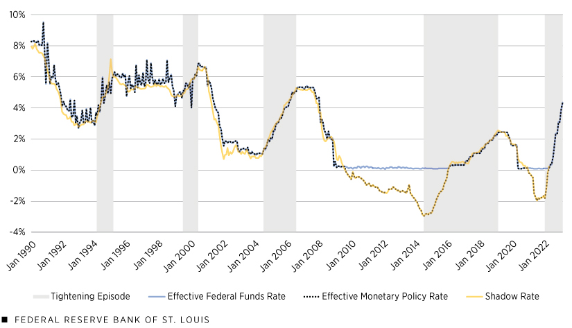
SOURCES: Board of Governors of the Federal Reserve System, “Measuring the Macroeconomic Impact of Monetary Policy at the Zero Lower Bound” (Wu and Xia, 2016) via the Federal Reserve Bank of Atlanta, and authors’ calculations.
NOTES: The effective federal funds rate and the shadow rate use end-of-month values. Data for the shadow rate are through the end of February 2022.
Personal Consumption Behavior across Episodes of Monetary Policy Tightening
The following figure shows how a measure of personal consumption expenditures (PCE) moves during the same tightening episodes (again indicated by the gray bars). The PCE measure (the blue line) is both in real terms (meaning that it is adjusted for inflation) and detrended (meaning that it is calculated as a percent deviation from its trend).This measure of percent deviation from the trend for consumption is given by applying the Christiano-Fitzgerald band-pass filter with a minimum period of three months and a maximum period of 96 months to logged real consumption expenditures. The purpose of a band-pass filter is to obtain the cycle by removing very short fluctuations (less than three months in this case) and the trend (more than 96 months in this case) from a time series. See Lawrence Christiano and Terry Fitzgerald’s NBER working paper “The Band Pass Filter” (PDF) for a more detailed explanation. We refer to this measure of consumption as the real consumption cycle. Negative values indicate lower-than-normal household consumption, while positive values indicate higher-than-normal consumption. For simplicity, we exclude the effective monetary policy rate reported in the previous figure, since the gray bars provide information about when the effective monetary policy rate is increasing.
Detrended Real PCE and Tightening Episodes, 1990-2022
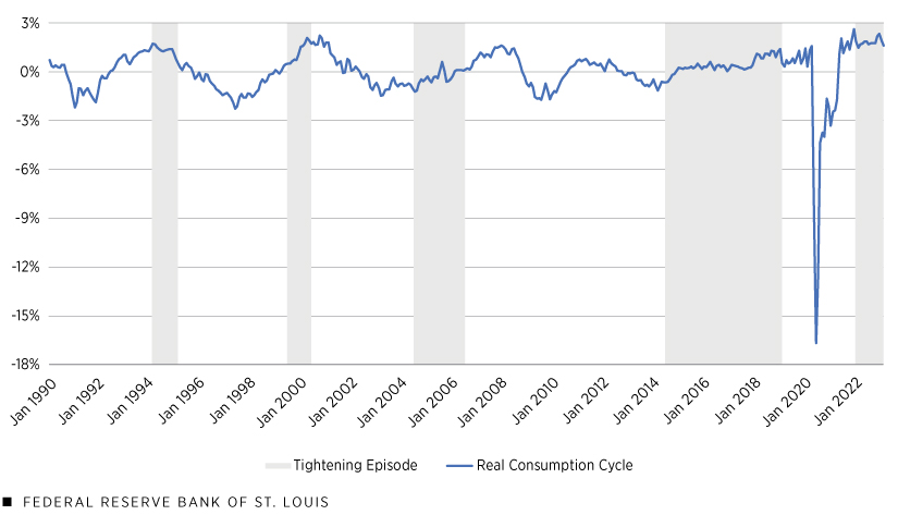
SOURCES: Bureau of Economic Analysis and authors’ calculations.
The above figure yields several observations. In the 1994 tightening episode, as the effective monetary policy rate began to rise (as indicated by the start of the gray bar), the real consumption cycle was at a peak. Then, as the effective monetary policy rate increased, real consumption declined and eventually became negative, indicating lower-than-normal consumption. This is exactly the pattern predicted by the theory we described at the start of our article. The pattern is similar, but delayed, in the subsequent tightening episode (1999); consumption began to decline 16 months after the tightening episode started.
In contrast, consumption increased in the 2004 tightening episode, and it stayed relatively close to its trend in the 2014 tightening episode. Thus, how the theory suggests that consumption should behave during periods of tightening monetary policy is not clearly observed in at least two of the first four tightening episodes in our analysis. The lockdowns and uncertainty associated with the COVID-19 pandemic rapidly reduced consumption in 2020. However, it returned to trend relatively quickly, before the most recent tightening episode began at the end of 2021.
Consumption and Financial Conditions during the 2021 Tightening Episode
The next figure focuses on the most recent tightening episode, the beginning of which is marked by the vertical dashed line. For simplicity, we included only the effective monetary policy rate as we previously defined it (the black line below) and excluded its effective federal funds rate and shadow rate components.
Monetary Policy Rate, Consumption and Financial Conditions, October 2020-December 2022
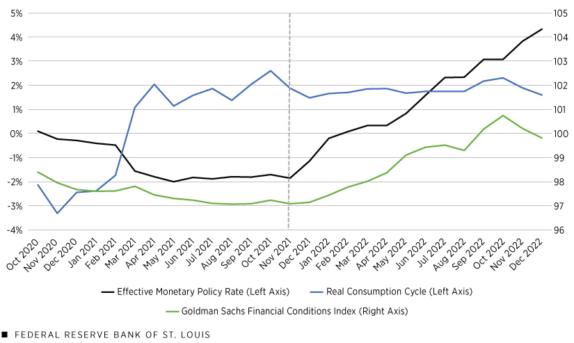
SOURCES: Board of Governors of the Federal Reserve System, “Measuring the Macroeconomic Impact of Monetary Policy at the Zero Lower Bound” (Wu and Xia, 2016) via the Federal Reserve Bank of Atlanta, and authors’ calculations.
NOTES: The effective monetary policy rate is the effective federal funds rate when positive and the Wu-Xia shadow rate when negative. Data are monthly. We report the monthly average of the Goldman Sachs Financial Conditions Index. An index value of 100 indicates average conditions.
As the figure illustrates, consumption as measured by the real consumption cycle (the blue line) declined slightly following the start of the 2021 tightening episode. Despite small fluctuations such as that, the real consumption cycle has consistently lingered about 2% above trend since the start of the tightening episode. The positive values of the real consumption cycle indicate that consumption was higher than normal. Slower growth in the last two months of 2022 supports the theory that tightening monetary policy decreases consumption, but this evidence is weakened by the fact that consumption remained higher than normal.
The green line represents a financial conditions index constructed by Goldman Sachs. A higher value on the index indicates that it is harder to borrow and invest, for example, because of higher borrowing costs for companies or lower equity prices. The index generally followed the movements in the effective monetary policy rate before and during the 2021 tightening episode; however, in the last two months of 2022, the index declined, meaning that financial conditions eased despite the Fed’s interest rate hikes. Since the beginning of the tightening episode, most months have registered average or better-than-average (an index value below 100) financial conditions, which may help to explain why consumption has remained elevated during this period.
In conclusion, there is some evidence, although weak and not recent, that the real consumption cycle declines during episodes of monetary policy tightening. In 2022, consumption remained approximately 2% above trend. Additionally, financial conditions—shown by the financial conditions index—improved at the end of 2022 despite the Fed tightening monetary policy. Looking toward the future, it may be important to track the correlation of the financial conditions index and the effective monetary policy rate, which have recently diverged, to predict the behavior of consumption and inflation.
Notes
- This logic is close to the description of the Phillips curve in this May 2020 working paper from the European Central Bank (PDF).
- Short-term rates are those with maturity less than one year. The federal funds rate is a short-term rate.
- See their paper, “Measuring the Macroeconomic Impact of Monetary Policy at the Zero Lower Bound,” published in the March 2016 issue of the Journal of Money, Credit and Banking.
- We focus on five tightening episodes. Their start dates are February 1994, June 1999, June 2004, May 2014 and November 2021.
- This measure of percent deviation from the trend for consumption is given by applying the Christiano-Fitzgerald band-pass filter with a minimum period of three months and a maximum period of 96 months to logged real consumption expenditures. The purpose of a band-pass filter is to obtain the cycle by removing very short fluctuations (less than three months in this case) and the trend (more than 96 months in this case) from a time series. See Lawrence Christiano and Terry Fitzgerald’s NBER working paper “The Band Pass Filter” (PDF) for a more detailed explanation.


Views expressed in Regional Economist are not necessarily those of the St. Louis Fed or Federal Reserve System.
For the latest insights from our economists and other St. Louis Fed experts, visit On the Economy and subscribe.
Email Us
