

How Will COVID-19 Affect the Spending of Financially Distressed Households?
The following is the third post in a series examining the potential impact of COVID-19 on people living in areas already experiencing above average levels of financial distress.
In our previous posts, we analyzed how public-health policies like social distancing and “shelter-in-place” orders will likely have varying employment and earnings consequences across the U.S.See our other posts in our COVID-19 and financial distress series, covering employment vulnerability and vulnerability to infection and death. In particular, we found that areas characterized by high financial distress are more likely to suffer employment and earnings losses because they tend to have higher employment shares in susceptible industries like “accommodation and food services.” Furthermore, we showed that the growth of COVID-19 cases was initially highest in areas with the least financial distress, but we predicted that more distressed areas would soon outpace the others in terms of both infections and deaths.These predictions have largely become true, as can be seen in our regularly updated data-series.
In light of how highly financially distressed areas may bear a disproportionate share of the economic harms because of COVID-19, this post will examine what that means for household spending (or “consumption”). To do this, we use a model (described in detail in our recent working paper) combined with the empirical results from our previous posts, and we arrive at the following conclusions: First, based on plausible measures of the likely earnings losses, our framework suggests that average consumer spending will drop substantially—around 3.3 percent. Second, and perhaps more important, these consumption declines are deeply unequal—hitting those living in areas of highest financial distress the hardest.
Modeling Household Balance Sheets and Financial Distress
Our model is ideal for this analysis because it features a rich description of household balance sheets and has clear channels through which financial distress manifests itself. In terms of balance sheets, households are allowed to accumulate credit card debt, save in the kinds of liquid and safe financial assets they can likely access in reality (e.g., savings account) and own houses, which are financed with mortgages. In terms of financial distress, our simulation-based approach is one in which households can become delinquent (i.e., delayed) on credit card payments, file for bankruptcy (which erases all financial debts) or default on their mortgages (i.e., enter into foreclosure).
Moreover, because income is uncertain, this model captures the decisions of households who are aware of the risk they face, and who then make spending and savings choices while taking that uncertainty into account.
To use the model to derive predictions for spending, we generate five artificial economies within our framework, each meant to model one of the quintiles of financial distress explained in our previous posts. Recall that the group we call Q5 is comprised of individuals who live in the 20% of ZIP codes that exhibit the highest levels of household financial distress. Similarly, the group that we call Q1 represents individuals who live in the 20% of ZIP codes that exhibit the lowest levels of household financial distress.
Our findings from previous posts and other empirical work provide a guide for determining the size of unexpected income losses across sectors and quintiles of financial distress. Our methodology is similar to our earlier On the Economy blog post, “How Closing Restaurants and Hotels Spills Over to Total Employment.” At an aggregate level, we assume final demand falls by 75% in the “accommodation and food” sector and in related sectors like “leisure and hospitality.” Using input-output tables provided by the Bureau of Labor Statistics (BLS), we can trace how this decline in demand translates into employment or earnings losses across sectors.
The input-output tables imply this aggregate shock translates into employment losses ranging from roughly 59% in the food and accommodation sector (which accounts for roughly 8% of total employment and is the hardest-hit sector) to virtually zero in sectors that aren’t affected by social distancing (which account for 40% of total employment). Sectors somewhere in the middle that are moderately affected by social distancing (accounting for 52% of total employment) experience 5% employment losses.This employment breakdown resembles the findings in Leibovici, Fernando; Santacreu, Ana Maria; and Famiglietti, Matthew. “Social Distancing and Contact-Intensive Occupations.” St. Louis Fed On the Economy Blog, March 24, 2020. They categorized occupations by how contact-intensive they are and hence how likely they are to be affected by social-distancing measures. Our numbers are larger because we account for spillovers across industries and occupations.
Finally, because each quintile of financial distress differs in its composition of employment, we can convert these sector-specific losses into losses for each quintile. For example, our previous posts show that the employment share in “accommodation and food” ranges from roughly 7% in the lowest quintile of financial distress, to nearly 11% in the highest quintile of financial distress. This suggests that a larger share of the population in high-distress areas are likely to receive larger earnings losses. The figure below shows the average earnings loss for each quintile implied by these assumptions:
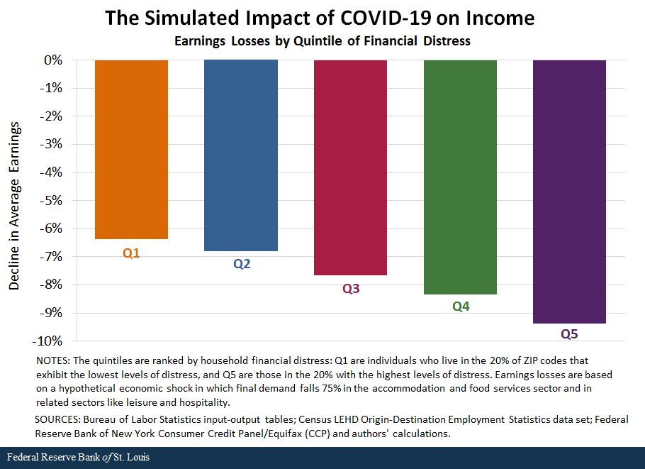
The next figure plots the change in spending and makes clear that financial distress is an important “preexisting” condition. (All numbers are in annual terms and are calculated as percentage changes relative to a baseline scenario in which the shocks never occur.) Comparing the two extremes, consumption falls by roughly 5% in Q5 (highest financial distress), which is more than double the fall measured in Q1 (lowest financial distress).
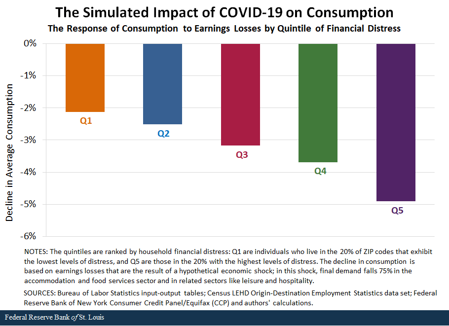
Importantly, the declines in consumer spending that we note above result from two combined effects: (1) regions with greater financial distress experience larger earnings losses because they have higher employment shares in “accommodation and food,” and (2) higher financial distress regions are more vulnerable (through “preexisting conditions”) to any shock. Using the machinery of our model, we can separate these two effects to see which is quantitatively more important.
Modeling the Effect of Financial Distress as a Preexisting Condition
To gauge the “pure” effect of financial distress as a preexisting condition, the figure below shows the spending responses across the financial distress spectrum under an alternative scenario wherein all regions experience the same earnings losses. We set these losses equal to those of Q1 (the lowest financial distress).
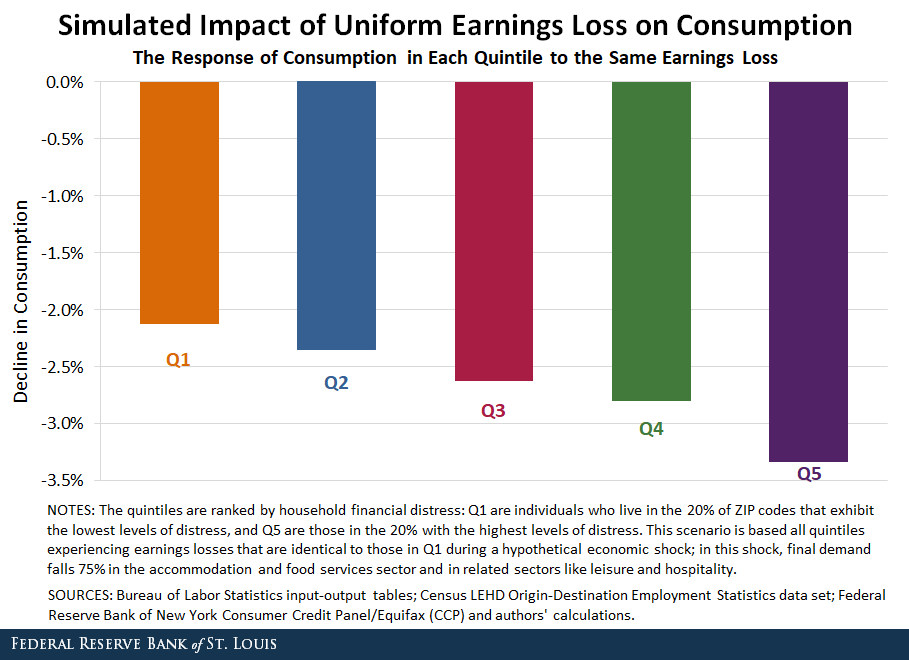
By construction, the Q1 bar in the last two figures is the same. However, all other bars are different, with the differences reflecting the direct effects of “preexisting” conditions in generating differential drops in spending. The bar for Q5 (the highest financial distress) in the third figure shows that when this region faces an earnings shock similar to Q1, their consumption still declines by over an extra percentage point relative to Q1 (i.e., 3.3% versus 2.1%).
This suggests that roughly 40% of the difference (which was 2.8 percentage points) in consumers’ spending response between Q1 and Q5—observed in the second figure—comes solely from preexisting conditions, while the other 60% occurs because those with the highest financial distress (Q5) experience larger earnings losses related to COVID-19.
Our results carry a more general lesson: The preexisting condition of “financial distress” that we emphasize will matter in a broad array of circumstances for income losses. To see this, consider the two lines of the table below, which show the ratio of the change in consumption compared with the change in income under both the baseline (Figure 2) and alternative (Figure 3) scenarios we study.
| Q1 | Q2 | Q3 | Q4 | Q5 | |
|---|---|---|---|---|---|
| Baseline | 0.33 | 0.37 | 0.41 | 0.44 | 0.52 |
| Alternative | 0.33 |
0.37 | 0.41 | 0.44 | 0.52 |
| Each cell plots the percentage change in consumption divided by the percentage change in earnings. The “Baseline” scenario follows the earnings losses by quintile plotted in Figure 1. Meanwhile, the “alternative” scenario sets all earnings losses across quintiles equal to those experienced by Q1. | |||||
Two points emerge: First, in both scenarios, those initially most distressed (Q5) are very vulnerable. Their spending drops roughly half a percentage point for each percentage point decline in income. In contrast, the least-distressed (Q1) reduce their spending by roughly a third of a percentage point for each percentage point decline in income. Interestingly, both rows have the same numbers, indicating that the elasticity in each financial distress group does not depend on the size of the shock.
For instance, Q5 has a reduction of income of 9% in the benchmark exercise and 6% in the uniform shock, and in both cases the elasticity is 0.52. This in part reflects the way we have imposed the shocks to income on the different groups, but is strongly suggestive that overall sensitivities (i.e., the proportional response of consumer spending to the change in their income) may not hinge on the size of the shock.
Second, and again in both scenarios, the response of spending is sizeable, reflecting the fact that the earnings shocks are hard to cope with.
Conclusion
Overall, our calculations strongly suggest that in response to the earnings losses that will plausibly accompany the social distancing response to COVID-19, consumer spending is likely to contract much more in areas that entered this episode with higher financial distress. Indeed, our numbers suggest that the decline in consumption will be over twice as large between the lowest and highest quintiles of financial distress. Part of this is related to the magnitude of the shock each region receives, but an equally large part is related to the “preexisting conditions” each region has.
What do these results imply for policy? In our view, the findings here mean that special consideration should be given to assessing the nature of financial distress when deciding on policies designed to mitigate or offset these earnings losses. This is especially true for any policies that are already tailored toward helping more financially distressed communities, as they are likely to be most at risk and least able to maintain their living standards.
In our next series of posts, we will use our model to examine the effects of some policy initiatives that take into explicit account differences in initial consumer financial distress.
Notes and References
1 See our other posts in our COVID-19 and financial distress series, covering employment vulnerability and vulnerability to infection and death.
2 These predictions have largely become true, as can be seen in our regularly updated data-series.
3 Our methodology is similar to our earlier On the Economy blog post, “How Closing Restaurants and Hotels Spills Over to Total Employment.”
4 This employment breakdown resembles the findings in Leibovici, Fernando; Santacreu, Ana Maria; and Famiglietti, Matthew. “Social Distancing and Contact-Intensive Occupations.” St. Louis Fed On the Economy Blog, March 24, 2020. They categorized occupations by how contact-intensive they are and hence how likely they are to be affected by social-distancing measures. Our numbers are larger because we account for spillovers across industries and occupations.
5 For example, our previous posts show that the employment share in “accommodation and food” ranges from roughly 7% in the lowest quintile of financial distress, to nearly 11% in the highest quintile of financial distress. This suggests that a larger share of the population in high-distress areas are likely to receive larger earnings losses.
Additional Resources
- St. Louis Fed’s COVID-19 resource page
- Timely Topics: Financial Distress and COVID-19
- On the Economy: COVID-19 and Financial Distress: Vulnerability to Infection and Death
- On the Economy: COVID-19 and Financial Distress: Employment Vulnerability


This blog offers commentary, analysis and data from our economists and experts. Views expressed are not necessarily those of the St. Louis Fed or Federal Reserve System.
Email Us
All other blog-related questions
